Chapter 3: Neural Networks

Beyond Linear Regression

Many statisticians have built upon the idea of linear regression to make it useful in different settings, like when our outcome is a probability between 0 and 1 (logistic regression) or when we want to assume that $f(X)$ is a polynomial (polynomial regression). There are multiple extensions, but the central concept is always the same: we specify how $X$ relates to $y$ and define some transformations to make the relationship linear.

As data has become increasingly complex, it has become harder and harder to specify the relationship between $X$ and $y$ a priori. In fact, we often want to learn the relationship itself. In small datasets, this is generally not possible, since there are an infinite number of functions $f$ relating $X$ to $y$ . But in large datasets, we can learn surprisingly effective approximations of the true $f$ . This is ultimately what neural networks are doing.

Neural Networks

You may be wondering why we discussed linear regression in so much detail, when we are really trying to understand the more advanced machine learning techniques. The secret is that neural networks are simply applying linear regression in sequence. Different architectures add different bells and whistles, but linear regression is the foundation.

So what are neural networks exactly? For this bootcamp, neural networks are prediction models built from interconnected layers of artificial neurons, as shown below. The key point is that each “artificial neuron” actually represents a linear regression model. Diagram of a neural network

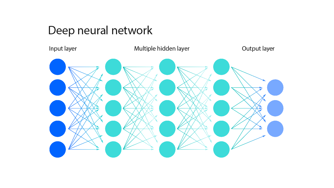
Importantly, neural networks are layered. We pass in our original data $X$ into the input layer, which is then transformed into the first hidden layer, which we will denote as $Z^{(1)}$ . This first hidden layer is transformed into multiple subsequent hidden layers ( $Z^{(2)}, \ldots, Z^{(d)}$ ), until we finally get a prediction for $y$ in the output layer.

To introduce the last piece of mathematical notation in this bootcamp, the equation for computing layer $d$ in a neural network is:

Z^{(d)} = W^{(d)} \cdot \sigma(Z^{(d-1)}) + b^{(d)}

where $Z^{(1)} = W^{(1)} X + b^{(1)}$ , and $\sigma$ is an activation function meant to mimic the electrical activation of biological neurons. You don’t need to worry too much about the details of the equation; the main idea is that computing each layer looks a lot like linear regression, with parameters $W^{(d)}$ and $b^{(d)}$ for each layer $d$ . In fact, linear regression is equivalent to a neural network with no hidden layers!

One basic interpretation of neural networks is that they transform your observations $X$ into a “hidden representation” via linear regression, then transform the hidden representation once more with another linear regression, and so on and so forth, until the final linear regression outputs a prediction for $y$ . The slight nuance is that we apply the activation function $\sigma$ after every regression. This step introduces non-linearity into our model, which allows us to approximate very complicated functions. In fact, neural networks with a single hidden layer are universal function approximators, meaning that any continuous function can be approximated arbitrarily well by a neural network.

Before moving on to large language models, it is worth elaborating a bit more on the purpose of a neural network’s layers. The number of layers in a neural network is referred to as the network’s depth. When people say that “deep learning” is currently the most powerful machine learning approach, they mean that deeper networks tend to be extremely effective at learning the relationship between the observations $X$ and the outcome $y$ .

We still don’t understand why deep neural networks are so good at this task, but their success seems to be related to the structure of the hidden layers. In particular, as we move to large language models, you can begin to think of the hidden layers as representing the internal state of the model: its thoughts, in some sense. As a network becomes deeper, its internal state becomes highly non-linear, allowing it to represent increasingly complicated ideas in its hidden layers. We’ll see how these hidden layers are translated to language in the next chapter.

Exercise: When should linear regression be preferred over a neural network?

Further Study

This video is the beginning of a phenomenal series on deep learning. This creator likes to go a little deep into some of the math, but his visualizations are fantastic. Definitely worth a watch.